| An optical processor lets us analyze an image and synthesize the image with various modification by optical means. A standard optical processor consists of two equal converging lenses with focal lengths f separated be a distance 2f. The image to be analyzed is placed in the object focal plane of the first lens and illuminated with coherent light incident parallel to the optical axis. An inverted image with unit magnification appears in the image focal plane of the second lens. This is the synthesized image and it can be manipulated and modified by placing masks and filters in the image focal plane of the first lens. This plane is called the frequency plane. It is also the object focal plane of the second lens. |
|
|
Why does this work? Assume the original image in the object focal plane of the first lens is a single slit. We have already calculated the Fraunhofer diffraction patter of a single slit. It is the far-field diffraction pattern of the slit, which can be projected by a converging lens into the focal plane of the lens. Fresnel's principle guaranties that the relative phases in the focal plane of the lens are equal to the relative phases for a focus at infinity. We found for the field amplitude a distance x'' from the optical axis
|
|
Converting to exponential notation we have
 .
.
Let
us define
kx'' = ksinθ ~ kθ.
We have x'' = f tanθ ~ fθ
and therefore x''
 kx''. We therefore write
 .
.
Here g(x) = 1, -a/2 < x < a/2, and g(x) = 0 everywhere else.
The electric field amplitude E(kx'') in the frequency plane (the image focal plane of the first lens) is proportional to the Fourier transform of of the field amplitude g(x) in the object focal plane of the first lens.
![]()
We have found that for the single slit the electric field amplitude E(kx'') in the frequency plane (the image focal plane of the first lens) is proportional to the Fourier transform of of the field amplitude g(x) in the object focal plane of the first lens. This not only holds for the single slit, but for any (real or complex) amplitude function g(x). If the field amplitude g(x,y) in the object plane of the first lens depends on two coordinates x and y, then the field amplitude in the frequency plane E(kx'',ky'') is proportional to the the two-dimensional Fourier transform of g(x,y). We can find the Fourier transform of a light distribution by optical means. Moreover, we can find the Fourier transform of the electric field distribution, not the intensity distribution, and thus preserve information about relative phases.
| For the single slit we have found the intensity pattern in the frequency plane. |
|
| The pattern <I(x'')> has the shape of the square of a sinc function. |
|
For the minima we have sinθ = mλ/a. Assume the diameter of the lenses of the optical processor is d. Because d is finite, the lens can only project M minima into the frequency plane. Light scattered at angles θ > θmax misses the lens. If the numerical aperture of the lens is NA = d/2f = sinθmax, then M = sinθmaxa/λ = da/(2fλ).
![]()
Let us now look at the second lens of the optical processor. From the field amplitude in the frequency plane it synthesizes an image in its image focal plane. The amplitude at a point a distance x from the optical axis is found by adding the contributions from all points in the frequency plane. If the first lens projects the complete diffraction pattern we have
If we let x' = -x then
Therefore
E(x') g(x), E(x') is the scaled Fourier transform of E(kx''), and kx''
is the wave number ("spatial frequency") of the component harmonic waves that add up to
produce g(x). The synthesized image is inverted, but otherwise identical to the original
image.
E(x'') extends to x'' = ±∞. But the magnitude of E(x'') decreases rapidly as x'' becomes large. If the diameter of the lens is large enough so that it intercepts a large number M of minima of the intensity distribution, then the synthesized image will be true to the original. We need M = (d/2f)(a/λ) >> 1 for the synthesized image to be true to the original.
We can modify the synthesized image by modifying the amplitude and phase of E(x'') in the frequency plane by optical means.
Assume we put an aperture in the frequency plane with diameter d' such that (d'/2f)(a/λ) ~ 1. We now restrict the range of "frequencies" kx'' which can contribute to the synthesized amplitude E(x'). (We only transmit the central maximum of the diffraction pattern and therefore implement a low-pass filter.) We have |kx''| < kd'/2f = kλ/a = 2π/a.
Let us choose our units so that a = 1. The E(kx'')= C sin(kx''/2)/(kx''/2) and

|
Using Microsoft Excels FFT function we find <I(x')> as shown on the right. The image now has smoothed edges and the intensity distribution across the image is no longer uniform. Spatial filtering is the manipulation of an image with masks in the frequency plane. Low-pass and high-pass filters are common spatial filters. A simple low-pass filter consists of a pinhole located on the optical axis in the frequency plane. It blocks all the high-frequency (short wavelength) components in the Fourier transform of the object. A simple high-pass filter consists of a small, opaque spot located on the optical axis in the frequency plane. It blocks all the low-frequency (long wavelength) components in the Fourier transform of the object. Link: The spreadsheet FFT2.xlsm is the same as FFT1.xlsm, except that it scales the FFT output to the size that would be obtained with an optical processor using 500 mm focal length lenses and 633 nm wavelength light. |
 |
Why does anyone build an optical image processor if it is so easy to manipulate digital images?
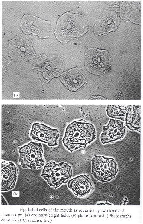
In ordinary microscopy, for example, most of the detail of living cells is undetectable because there is too little contrast between structures with similar transparency and there is insufficient natural pigmentation. Edge enhancement of the digital images does not work, because the images are very smooth. However the various organelles show wide variation in index of refraction. These index of refraction variations can be transformed into brightness variations by means of phase contrast microscopy.
Phase contrast microscopy uses phase plates, which when placed in the frequency plane change the phase of the low-frequency components by π/2, while leaving the phase of the high frequency components unchanged.
Assume a sample is transparent and only changes the phase of the transmitted wave by a small amount because of small index of refraction changes.
Aexp(i(kz-ωt)) --> Aexp(-iδ(x))exp(i(kz-ωt))
If δ(x) is small (δ(x)
<< 1) the transmitted amplitude may be written as A(1- iδ(x)).
The Fourier transform of such a function contains a large central peak around k
= 0 representing the constant term and much smaller peaks at larger values of k
representing the small variations δ(x). The
synthesized image amplitude is A(1- iδ(x')) and the
image intensity is
|A(1- iδ(x'))|2 = A2(1 + δ(x')2) ~ A2.
Assume we use a quarter wave plate in the frequency plane (the focal plane of a lens) to change the phase of the central spot by exp(-iπ/2) = -i. The synthesized image amplitude then is approximately A(-i - iδ(x')) = -iA(1 + δ(x')) and the image intensity is
|iA(1+ δ(x'))|2 ~ A2(1 + 2δ(x'))
The phase contrast has been converted into an amplitude contrast and the object becomes visible.
Link: The Excel spreadsheet FFTphase.xlsm from above with a phase contrast button.
Here is a MATLAB Simulation. Import the scripts to your MATLAB folder.
 .
.