In this laboratory you will study some aspects of the random nature of radioactive decay.  You will verify that if the count rate is low, the probability of recording a particular number of counts is given by the Poisson distribution, and that if the count rate is high, the probability of recording a particular number of counts is given by the Gaussian distribution.

You will observe that when counting random events, the actual number of counts recorded (N) is often very different from the average number of counts recorded (N).  Approximately 1/3 of the time the actual number of counts N will differ from the average number of counts N by more than the standard deviation σ = N^1/2.   The relative standard deviation σ/N = N^-1/2 decreases as N increases.  When counting a large number of random events the percentage difference between the  actual number of counts N and the average number of counts N is likely to be much smaller and the measurement will have a much higher statistical significance than when counting a small number of random events.

Background information:

There are many types of events that that occur at a well defined average rate, but for which we cannot predict the outcome of any particular measurement.  For example, a light bulb has an average lifetime.  But we cannot predict how long a particular light bulb will last.  This is a characteristic of a random process.  A random variable is a function that associates a unique numerical value with every outcome of an experiment.  The value of the random variable will vary from trial to trial as the experiment is repeated.  For the light bulb the experiment is measuring its lifetime, and the random variable is the number of days it produces light before it burns out.

The average number of rain days in May in Nashville is 11.  We cannot predict how many rain days Nashville will have next year in May and on which days it will rain.  If we record the number of rain days next May, the new number will most likely differ from that of the preceding May.  The number we will record cannot be predicted using the knowledge of a preceding observation nor can it be used to predict the following observation. 

Radioactive decay is a random process.  We cannot predict exactly when a certain unstable nucleus will decay, we can only predict the probability that the nucleus will decay in a certain time interval.  Similarly, we cannot predict exactly how many decays will take place in a particular radioactive sample in a particular time interval, but only the average number of decays.  If we actually count the number of decays in several time intervals, we get a different number of counts each time, but they have a more or less definite mean.

Assume we count the number of times N a given random event occurs in a certain time interval.  Statistical theory predicts that if we repeat our experiment m times, we will find the numbers N₁, N₂, N₃, ..., N_m.  We can calculate the average number of counts N = [Σ₁^m N_i]/m.  The actual number of counts will be distributed around this average value.  Numbers close to the average will be recorded frequently, numbers very different from the average will be recorded infrequently. If we want to know how the actual number of events counted in a time interval ∆t is distributed around the average number of events counted in ∆t, we can make  histogram of the number of times a certain number N appears. 

For a large number of rare events we find that the probability of recording a particular number N is given by the Poisson distribution:

P(N) = N^N exp(-N)/N!

The Poisson distribution describes a wide range of phenomena in the sciences.  It describes the probabilities of random occurrences and it can be applied to  "intervals" on the space or time axes.

For a large number of frequent events we find that the probability of recording a particular number N is given by the Gaussian distribution:

P(N) = [1/(2πN)]^1/2 exp[-(N-N)²/(2N)]

For a large N the Poisson distribution approaches the Gaussian distribution.

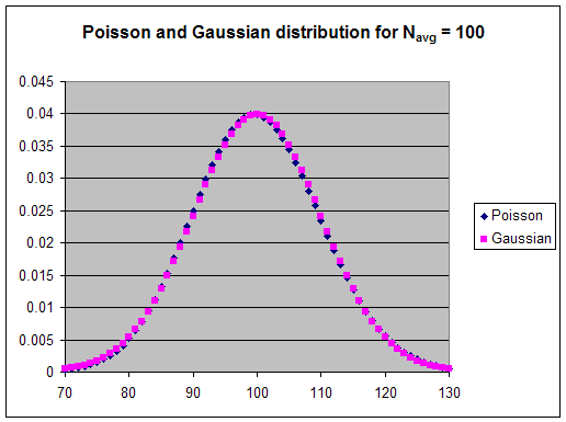
Statistical theory predicts that the standard deviation of the Gaussian distribution is given by σ = N^1/2.  The standard deviation σ is a measure of the width of the distribution.  Approximately 1/3 of the counts will lie outside the interval  N - σ to N + σ.

The standard deviation is calculated using

 .
 

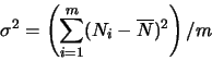Equipment needed:

• Geiger Tube with Stand and Source Holder
• Nucleus Scaler/Timer
• Pasco Science Workshop 750 Data Acquisition System
• BNC to Phone Plug Cable
• Sr and Cs Radioactive Sources

The Geiger-Mueller (GM) tube is a simple device for detecting radiation.  It is a gas-filled metal cylinder (the cathode) with a wire (the anode) running down its axis.  The wire is insulated from the cylinder.  A high-voltage establishes a potential difference between the anode and the cathode.  The anode potential is positive with respect to the cathode potential.  The resulting electric field inside the cylinder has its largest magnitude near the anode.

When a alpha or beta particle or gamma-ray passes through the cylinder, it ionizes some of the gas, removing  the outermost electrons from some of the gas atoms.  These electrons are accelerated towards the anode by the electric field, and quickly gain enough kinetic energy to ionize more gas atoms.  An avalanche of electrons reaches the anode and produces a pulse large enough to be detected.

The Geiger tube is mounted vertically in a stand.  The Pasco Interface receives the pulses from the GM tube and transfers data to the PC.

Procedure:

Part 1:

• Make sure the Science Workshop Interface (SW) is on.
• Connect the Geiger-Mueller tube to the Nuclear Scaler/Timer and the Scaler/Timer to the Science Workshop interface.  Insert the phone plug to digital channel 1 of the interface.
• Make sure the high voltage for the scaler is set to 900 V, and the counting mode switch is set to Preset Time, Manual.
• Place the source near the bottom of the source holder.
• Turn on the scaler.  Place it into stop mode by pressing the Stop and then the Reset switch.  Then press count.  It should start counting.
• Open Data Studio and choose to create an experiment.
• Click on the circle for channel 1 and add a Geiger counter.  Choose sample rate 5 Hz.
• Click "Sampling Options".  Choose Delay Start, None.  Choose Automatic Stop, Time, and set the time to 500.2 s.  This will allow 2500 measurements in 0.2 s increments.  Click "OK". 
• Minimize the "Experiment Setup" window.
• From the "Displays" double click the graph icon.  This will display the data collected from the Geiger counter in a graph.
• Click Start and start collecting data.
• Observe the number of events detected in 0.2 s.  Move the source to a position that yields an average number of 5 -15 counts.
• Click Stop.  Select Experiment from the menu bar and then Delete All Data Runs from the pull-down menu.
• Click Start and collect data for the next 500 s.

Part 2:

• Click Start and start collecting data.
• Observe the number of events detected in 0.2 s.  Move the source to a position that yields an average number of 100 - 200 counts.
• Click Stop.  Select experiment from the menu bar and then Delete Last Data Run from the pull-down menu.
• Click Start and collect data for the next 500 s.

Data Analysis:

Part 1:

• Click the statistics button (the Σ symbol) on your graph.  Choose Min, Max, Mean, and Std Dev.  These quantities will be displayed on the graph.
• From the "Displays" drag the histogram icon onto Run #1.  A histogram of your data will be displayed.
• Double click on the histogram.  A Histogram Settings window will open.  Click bins, specific bins, starting bin = 0, bin size = 1.  Click ok.
• Click the icon in in the upper left corner of the histogram to auto-scale the graph.  The histogram now displays the frequency f of a particular number N of counts in a 0.2 s time interval is plotted versus N.
• Open an Excel spreadsheet.
• In Data Studio highlight your histogram and click edit copy.  In Excel go to cell A1 and click edit, paste.  This transfers the data to Excel.
  Unfortunately Data studio labels the bin containing N counts by N - 1.  If we want to plot the number of times we observed N counts versus N, we have to increase the values in column A by 1.
  Into column C3 type =A3+1, and copy this formula into the cells below.
  Highlight the values in column C, click edit, copy.  Then highlight cell A3 and click edit, paste special, values.  Now delete column C.
• The Poisson distribution give the he probability of recording a particular number N of counts. 

  P(N) = N^N exp(-N)/N!

  Since we made 2500 measurements, 2500*N^N exp(-N)/N! is the number of times we expect to record N counts.  Into column C enter the formula for the expected distribution.
  Type = 2500*N^A3*exp(-N)/Fact(A3) into cell C3, where N is the mean Data Studio calculated for you.  Copy the formula into the remaining cells of column C.

• Plot columns B and C versus column A.  Compare the graph of the actual and expected frequencies f.

Part 2:

• From the "Displays" drag the histogram icon onto Run #2.  A histogram of your data will be displayed.
• Double click on the histogram.  A Histogram Settings window will open.   Click bins, specific bins, starting bin = 0, bin size = 1.  Click ok.
• Click the icon in in the upper left corner of the histogram to auto-scale the graph.  The histogram now displays the frequency f of a particular number N of counts in a 0.2 s time interval is plotted versus N.
• In Data Studio highlight your histogram and click edit copy.  In Excel go to cell E1 and click edit, paste.  This transfers the data to Excel.
  Increase the values in column E by 1, as described in part 1.
• The Gaussian distribution give the he probability of recording a particular number N of counts. 

  P(N) = [1/(2πN)]^1/2 exp[-(N-N)²/(2N)]

  Since we made 2500 measurements, 2500*[1/(2πN)]^1/2 exp[-(N-N)²/(2N)] is the number of times we expect to record N counts.  Into column C enter the formula for the expected distribution.
  Type = 2500*(2*pi()*N)^(-1/2)*exp(-((E3-N)^2/(2*N)))  into cell G3, where N is the mean Data Studio calculated for you.  Copy the formula into the remaining cells of column C.

• Plot columns F and G versus column E.  Compare the graph of the actual and expected frequencies f.

Open Microsoft Word and prepare a report.

Name:
E-mail address:

Laboratory 7 Report

• Summarize the experiment.

• Insert your Excel graphs and discuss your results.  In the discussion you should answer the following questions.

  • For part 1, what was the average number of counts in a 0.2 s time interval?

  • What is the formula for the expected distribution?

  • Does a plot of f versus N resemble the expected distribution?

  • For your measured distribution what is the ratio of the full width at half maximum (FWHM) to the average?  Why might you be interested in this value?

  • For part 2, what was the average number of counts in a 0.2 s time interval?

  • What is the formula for the expected distribution?

  • Does a plot of f versus N resemble the expected distribution?

  • For your measured distribution what is the ratio of the full width at half maximum (FWHM) to the average?  Why might you be interested in this value?

• Add any comments or questions you may have.