More Problems

Problem 1:

Suppose an electron is in a state described by the wave function

ψ = (1/√4π)(e^iφsinθ + cosθ)g(r),

where  ∫₀^∞ |g(r)|²r²dr = 1, and φ, θ are the azimuth and polar angles respectively.

(a)  What are the possible results of a measurement of the z-component L_z of the angular momentum of the electron in this state?
(b)  What is the probability of obtaining each of the possible results in part (a)?
(c)  What is the expectation value of L_z ?

Solution:

• Concepts:
  The spherical harmonics, the postulates of quantum mechanics
• Reasoning:
  If we want to find the probability of measuring the eigenvalue a of an observable A we must express the wave function of the system as a linear combination of eigenfunctions of A.  Then P(a) = Σ_i|<aⁱ|ψ>|².
  Express the wave function in terms of spherical harmonics.
  Y_1±1 = ∓(3/8π)^½sinθ exp(±iφ),  Y₁₀ = (3/4π)^½cosθ.
• Details of the calculation:
  (a)    ψ = (1/3)^½(-√2 Y₁₁ + Y₁₀)g(r),  the possible results for a measurement of L_z are 0 and ħ.
  (b)    The wavefunction ψ is normalized.  The probability of measuring 0 is 1/3, the probability of measuring ħ is 2/3.
  (c)     The expectation value <L_z> = 0*P(0) + ħP(ħ) = (2/3)ħ.

Problem 2:

Let the matrices S_x and S_y be the matrices of an operator in some basis.

(a)  What is the spin quantum number s of the particle?
(b)  Use the commutation relations [S_i,S_j] = ε_ijkiħS_k  to compute the matrix of S_z in that basis.
(c)  Find the normalized eigenvectors of S_x in that basis and show that they are orthogonal.

Solution:

• Concepts:
  Matrix multiplication, finding the eigenvalues of a matrix
• Reasoning:
  [S_x,S_y] = S_xS_y - S_yS_x = iħS_z,  det(S_x - λħI) = 0.
• Details of the calculation:
  (a)  A 3 by 3 matrix implies that the spin quantum number is 1.
  (b)  [S_x,S_y] = S_xS_y - S_yS_x = iħS_z.
   
  (c)  The eigenvalues of S_x are ½ħλ.
  
  
  λ = 0, ±2.  So the eigenvalues of S_x are ħ, 0, and -ħ.
  The corresponding normalized eigenvectors (up to a factor e^iφ) are given below.
  
  
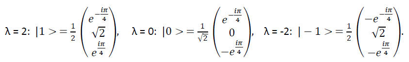
  <1|1> = <0|0> = <-1|-1> = 0. The vectors are normalized.
  Check: <1|0> = ½ *1/√2(1 - 1) = 0. <1|-1> = ¼(- 1 + 2 -1) = 0. <0|-1> = ½ *1/√2(-1 + 1) = 0.
  The vectors are orthogonal.

Problem 3:

A one-dimensional potential well is given in the form of a delta function at x = 0,
U(x) = Cδ(x), C < 0.  Find the energy and wave function of the ground state of the system. 

Solution:

• Concepts:
  This is a "square potential" problem.  We solve HΦ(x) = EΦ(x) in regions where U(x) is constant and apply boundary conditions.
• Reasoning:
  U(x) = 0 everywhere except at x = 0.
• Details of the calculation:
  E < 0.
  Φ₁(x) = A₁ exp(ρx) + A₁'exp(-ρx) for x < 0.  ρ² = -2mE/ħ².
  Φ₂(x) = A₂ exp(ρx) + A₂'exp(-ρx) for x > 0.
  Φ is finite at infinity.  If we choose ρ > 0, then A₁' = A₂ = 0. 
  Φ is continuous at x = 0.  Φ₁(0) = Φ₂(0).  A₁ = A₂' = A.
  
  ∂Φ/∂x has a finite discontinuity at x = 0.
  ∂²Φ(x)/∂x² + (2m(E - U)/ħ²)Φ(x) = 0.
  Let us evaluate this equation at x = ε and at x = -ε and write down a difference equation.
  ∂Φ_2ε(x₁ + ε)/∂x - ∂Φ_1ε(x₁ - ε)/∂x = -(2m/ħ²)∫_x1-ε^x1+ε (E - Cδ(x)) Φ(x) dx
  = (2mC/ħ²)Φ(0).
  ∂Φ₂/∂x|_x=ε = ∂Φ₁/∂x|_x=-ε + (2mC/ħ²)Φ(0), as ε --> 0.
  -ρA - (2mC/ħ²)A = ρA,  ρ = -mC/ħ².
  m²C²/ħ⁴ = -2mE/ħ²,  E = -mC²/(2ħ²).
  The wave function is Φ(x) = Aexp(-ρ|x|).
  Only one bound state exists.