
Consider a solid body consisting of a large number of atoms whose equilibrium positions are regularly arranged in a crystalline lattice. To treat such a solid quantum mechanically, we invoke the Born-Oppenheimer approximation. We attempt to solve the Schroedinger equation for the electrons for fixed positions of the nuclei. We try to solve for the electronic energy Eel(rq), where rq denotes the displacement of nucleus q from its equilibrium position. After finding Eel(rq) we try to solve the Schroedinger equation for the nuclei, assuming their potential energy U(rq) is given as the sum of their electrostatic interaction energy and Eel(rq). The nuclei are bound to their equilibrium positions by restoring forces. Expanding U(rq) in powers of rq and keeping only the lowest order non-vanishing terms we can treat the nuclei as a collection of coupled 3-dimensional harmonic oscillators.
Let us simplify and consider a one-dimensional problem, an infinite chain of one-dimensional coupled harmonic oscillators with potential energy
![]()
Here xq is the displacement of the qth nucleus from its equilibrium position, which we denote by ql. If the chain is infinitely long then the Hamiltonian is
![]()
In classical mechanics we can obtain the equations of motion from the Lagrangian
![]()
The equations of motion are
![]()
We can find real solutions
![]()
if
![]()
In these solutions all the oscillators vibrate with the same frequency ![]() and with the same amplitude 2|a|,
but with a phase that depends periodically on their equilibrium position. The
displacements are determined by a progressive sinusoidal wave of wave vector k and
phase velocity
and with the same amplitude 2|a|,
but with a phase that depends periodically on their equilibrium position. The
displacements are determined by a progressive sinusoidal wave of wave vector k and
phase velocity ![]() Two different values
of the wave vector k and k’ which are related through
Two different values
of the wave vector k and k’ which are related through ![]() lead to the same motion of the
oscillators, since
lead to the same motion of the
oscillators, since ![]() Waves with k’ and k are therefore physically
indistinguishable. To obtain the most general solution it is sufficient to let k
vary over an interval of
Waves with k’ and k are therefore physically
indistinguishable. To obtain the most general solution it is sufficient to let k
vary over an interval of ![]() This interval
is often called the first Brillouin zone.
This interval
is often called the first Brillouin zone.
Let us define new dynamical variables
![]()
Then
![]()
![]()
We therefore have
![]()
i.e. the evolution of Q(k,t) is independent of that of Q(k’,t) if k is not equal to k’. We have defined uncoupled variables, called normal modes. They can be defined so easily because we have an infinite chain, and therefore the system is invariant under a translation by an amount ±l. Real systems are not infinite in extend. But often we are interested in their behavior far from the edges, which we believe to be nearly independent of "edge effects". We then impose periodic boundary conditions, i.e. we assume that the two ends of the oscillator chain behave as if they were connected to each other. In the Lagrangian, we then sum from q=0 to q=N-1, where N is the number of oscillators. We require xN=x0. Solutions of the above form are then still obtained, but only for discrete values km=(2p)/(mL), m=1,2,...,N. If the chain is very long, then these values are very closely spaced.
Let us concentrate on the infinite chain. The variable ![]() is a periodic
function of k of period 2p/l, it is a
Fourier series whose coefficients
is a periodic
function of k of period 2p/l, it is a
Fourier series whose coefficients ![]() are
the displacements of the oscillators.
are
the displacements of the oscillators.
[Fourier transform: If f(x+L)=f(x), then f(x) can
be written as ![]() , with
, with  , where kn=n2p/L.
Here we have Q(k)=Q(k-2p/l), therefore we let f®Q, x®k, L®-2p/l, n®q, and kn®-ql.
The Bessel Parseval Relation:  ]
]
If we define
![]()
with
![]()
then we may write the Hamiltonian as
![]()
Here we have used the Bessel-Parseval relation
![]()
![]()
To make the transition from classical to quantum mechanics we let the classical canonical variables become operators. Defining
![]() and
and ![]()
and using [xq,pq']=i(h/2p)dq,q' we establish the commutation relations
![]()
We can therefore treat Q(k) and P(k) as operators corresponding to new canonical variables. Then
![]()
is a harmonic oscillator Hamiltonian. We define
![]()
where ![]() We find
We find
![]()
![]()
We may now write
![]()
In our problem a and aT are annihilation and creation operators analogous to those defined in the harmonic oscillator problem. But because k is a continuous index the commutator involves the delta function instead of the Kronecker delta.
The total Hamiltonian is the integral of the Hamiltonians for each of the normal modes.
The energy in each mode is quantized in units of ![]() W(k)=|2wsin(kl/2)|.
The ground state of the system is |0>, such that a(k)|0>=0 for all k.
The other stationary states of the system can be obtained by operating with aT(k)
on |0>. Each of the energies is an integral of the energies of each of the
modes. For a finite chain each of the energies is the sum of the energies of each of the
modes. For an infinite system the ground state energy is infinite, for a real system,
however, it is finite. We can then define the zero of our energy scale such that it is set
equal to zero.
W(k)=|2wsin(kl/2)|.
The ground state of the system is |0>, such that a(k)|0>=0 for all k.
The other stationary states of the system can be obtained by operating with aT(k)
on |0>. Each of the energies is an integral of the energies of each of the
modes. For a finite chain each of the energies is the sum of the energies of each of the
modes. For an infinite system the ground state energy is infinite, for a real system,
however, it is finite. We can then define the zero of our energy scale such that it is set
equal to zero.
In a crystal each of the vibrational normal modes is characterized by a wave vector k
and an angular frequency W(k). In solid state physics
the energy quantum associated with a mode is called a phonon.
The phonons are considered quasi-particles of energy ![]() and momentum
and momentum ![]() Phonons can be created and destroyed by adding to or taking from the
crystal the corresponding vibrational energy. In a finite system there exists a minimum
phonon energy
Phonons can be created and destroyed by adding to or taking from the
crystal the corresponding vibrational energy. In a finite system there exists a minimum
phonon energy ![]() The crystal cannot
exchange vibrational energy with its environment in smaller packages.
The crystal cannot
exchange vibrational energy with its environment in smaller packages.
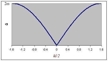
W(k)=|2wsin(kl/2)| is
the dispersion relation. It gives the possible phonon energies in terms of their momentum ![]() It gives the precise energies and momenta
that a crystal can absorb when it interacts with its environment. We can interpret
inelastic scattering of light by a crystal as the destruction or creation of a
phonon. The
energy and momentum of the incident photon has to change in such a way that the total
energy and momentum are conserved. The dispersion relation can also be interpreted as
giving the phase velocity
It gives the precise energies and momenta
that a crystal can absorb when it interacts with its environment. We can interpret
inelastic scattering of light by a crystal as the destruction or creation of a
phonon. The
energy and momentum of the incident photon has to change in such a way that the total
energy and momentum are conserved. The dispersion relation can also be interpreted as
giving the phase velocity ![]() and group
velocity
and group
velocity ![]() for
wave packets propagating
through the crystal. If
for
wave packets propagating
through the crystal. If ![]() then W(k)=wkl=vsk.
The phase
and group velocities are equal to vs=wl,
there is no dispersion. But when
then W(k)=wkl=vsk.
The phase
and group velocities are equal to vs=wl,
there is no dispersion. But when ![]() no
longer holds then the medium becomes dispersive, the group velocity is no longer equal to
the phase velocity. As
no
longer holds then the medium becomes dispersive, the group velocity is no longer equal to
the phase velocity. As ![]() the group
velocity goes to zero, a wave packet does not propagate.
the group
velocity goes to zero, a wave packet does not propagate.
Let us consider a stretched string of length L with two fixed ends. On a microscopic scale a string is not really continuous but we treat it as a substitute for some continuous quantity, such as the electromagnetic field. If we confine ourselves to small displacements from the equilibrium position u(x,t), then the partial differential equation satisfied by u is
![]()
Here F is the tension and m is the mass per unit length. Let
![]()
The fk satisfy the same boundary conditions as u(x,t), fk(0)=fk(L)=0, and the orthonormalization relation
![]()
We also have
![]()
Any function defined in the interval (0, L) which goes to zero at x=0 and x=L can be expanded in terms of the fk. We can therefore write
![]()
with
![]()
If we substitute ![]() into the equation
of motion we obtain
into the equation
of motion we obtain
![]()
The qk are the normal modes. They are decoupled and evolve independently.
The Hamiltonian of the system is H=T+V.
![]()
The potential energy for small displacements is
![]()
Therefore
![]()
This yields the Hamiltonian
![]()
with
![]()
To make the transition to quantum mechanics we let qk and pk
become operators. We then have ![]() i.e.
H is the sum of harmonic oscillator Hamiltonians. The eigenstate of H are
i.e.
H is the sum of harmonic oscillator Hamiltonians. The eigenstate of H are
![]()
The eigenvalues of ![]() If we choose the
energy of the |0,0,0,...> state as the zero of our energy scale, then
If we choose the
energy of the |0,0,0,...> state as the zero of our energy scale, then ![]() However the energy of the ground state is
infinite, so we are doing some hand waving here. We can also define the creation and
annihilation operators ak and akT.
However the energy of the ground state is
infinite, so we are doing some hand waving here. We can also define the creation and
annihilation operators ak and akT.
Energy is added or given up by the system only in units of ![]() In the state vector of the system,|n1, n2, n3,
...>, nk
then changes by ±1. In a quantized system the displacement u(x,t)
becomes the observable
In the state vector of the system,|n1, n2, n3,
...>, nk
then changes by ±1. In a quantized system the displacement u(x,t)
becomes the observable
![]()
The average value of this observable is
![]()
The average value for the ground state is <0|u(x)|0>=0. However <0|u2(x)|0>¹0. If we look at the displacement of the string as a substitute for the amplitude of some field quantity, such as the electric field, we conclude that even in the absence of any photons in the ground state of the field we have a non zero root mean square deviation of the amplitude. The vacuum state of the photons is subject to fluctuations of the field, called vacuum fluctuations. These vacuum fluctuations are responsible for the spontaneous emission of photons during the decay of excited atomic states. If we treat the electromagnetic field classically, then, if there is no field present, it cannot interact with exited atomic states, and these states are predicted to be stable. The vacuum fluctuations provide the coupling between field and atomic system necessary for the decay. Another effect of the vacuum fluctuations is to slightly modify the energy levels of atomic electrons. The Lamb Shift observed in the hydrogen atom spectrum is a consequence of this modification.
The operator u(x) and the Hamiltonian H do not commute. The displacement and the total energy are therefore incompatible observables. When referring to the electromagnetic field it is therefore impossible to know simultaneously the number of photons and the amplitude of the electric field at any point in space.