Fourier Transform Optics

Digital image processing lets us perform operations such as background subtraction, noise reduction, contrast enhancement, filtering, etc. on a digitized image, consisting of a rectangular array of numbers. One of the operations we can perform is Fourier transform filtering.

A digital image records light intensity as a function of position. According to Fourier's theorem any reasonably continuous function defined over some distance L can be synthesized by a sum of harmonic (sine and cosine) functions whose wavelengths are integral submultiples of L, (such as L/2, L/3, ...). Let f(x) be such a periodic function. Then we may write

f(x) = A₀/2 + ∑_n=1^∞ A_ncos(k_nx) + ∑_n=₁^∞ B_nsin(k_nx)

or f(x) = ∑_-_∞^+∞C_nexp(ik_nx),

where the coefficients A₀, A_n, and B_n or C_n can be calculated efficiently using computer algorithms. The k_n= n2π/L are equal to 2π times "frequencies" of the component harmonic waves. We actually do not sum over infinitely many frequencies, but only over frequencies up to the sampling frequency.

Review of the mathematical properties of the Fourier series and the Fourier transform.

Link: Making Waves Click on "Run Now" to explore how to synthesize various functions using only sine and cosine waves. The amplitude versus frequency plot tells us the amplitude (how much) of each sine and cosine function we have to use to reproduce the chosen function. This is called a plot of the function in the "frequency domain".

The Fourier transform of a two-dimensional image is a two-dimensional array of complex numbers giving the coefficients C_n. It is an important image processing tool. It represents the image in the frequency plane, i.e. each point represents a particular frequency contained in the image plane. We can now manipulate the transform in the frequency plane and observe how this affects the synthesized image in the image plane. Image filtering, smoothing, and edge enhancement are some of the effects we can achieve by manipulation the Fourier transform.

Examine the simple image of a square and its Fourier transform below.

Image

Fourier transform

The center of the Fourier transform plot represents the amplitudes of the low frequency sine and cosine waves that make up the image, while the outer regions represent the high frequency waves.

A low-pass filter eliminates all the frequencies above a cutoff frequency. If we synthesize the image using only waves with low frequencies (long wavelengths), then sharp features are no longer resolved. We have smoothed the image.

Applying a low-pass filter to the Fourier transform

The resulting smoothed image

A high-pass filter eliminates all the frequencies below a cutoff frequency. If we synthesize the image using only waves with high frequencies (short wavelengths), then smooth features of the image are largely eliminated and the sharp edges dominate. We have edge-enhanced the image.

Applying a high-pass filter to the Fourier transform

The resulting edge-enhanced image

This interactive tutorial lets you manipulate the Fourier transform. You can construct low-pass and high pass filters to smooth the image or produce edge enhancement effects.

Monochromatic optical images record light-intensity variations. The light intensity is proportional to the <E²>, the time-averaged square of the electric field vector.

Example:

In one dimension, consider a function f(x) = |f(x)| exp(iφ(x)). Assume that the intensity f(x) has been measured at N = 1024 evenly spaced points over a range from x = 0 to x - 10.24 mm. The sampling "frequency" therefore is 1/(0.01) mm = 100 mm^-1. The intensity I(x) = |f(x)|² is plotted on the right.

Let us find the discrete Fourier transform of this function using Microsoft Excel's FFT function.

The Fourier Analysis tool is a part of the Analysis ToolPak. It can be used to analyzes periodic data by using the Fast Fourier Transform (FFT) method to transform the data. This tool also supports inverse transformations, in which the inverse of transformed data returns the original data. The tool can be used to analyze one-dimensional data. To access the tool click "Tools, Data Analysis, Fourier Analysis" on Excel's toolbar.

How does it work?

Excel works with discrete data. One can define a Fourier transform for a discrete series of points called the discrete Fourier transform (DFT). Excel has a build in Fast Fourier Transform (FFT) algorithm. The FFT is simply a DFT that is faster to calculate on a computer.

Assume that we have a periodic function with period L which we are sampling at N discrete points.

f(x_n) = ∑_-_∞^+∞C(k_m)exp(ik_mx_n) ~ ∑_m=0^N-1C(k_m)exp(ik_mx_n)
C(k_m) = (1/L)∫₀^Lf(x)exp(-ik_mx)dx ~ (1/L)∑_n=0^N-1f(x_n)exp(-ik_mx_n)Δx.
Here k_m= m2π/L and Δx = L/N.
Therefore
f(x_n) = ∑_m=0^N-1C(k_m)exp(i2πmx_n/L)
C(k_m) = (1/N)∑_n=0^N-1f(x_n)exp(-i2πmx_n/L)

If we choose our units so that L = 1 and x_n = n(L/N) = n/N and k_m= m2π, then we can write

f(n) = ∑_m=0^N-1C(m)exp(i2πmn/N)
C(m) = (1/N)∑_n=0^N-1f(n)exp(-i2πmn/N)

0 ≤ n ≤ N-1, 0 ≤ m ≤ N-1

[We have N (complex) equations and N (complex) unknowns, a system that can be solved exactly.]

For N = 2ⁿ data, Excel's FFT and inverse FFT implement the relationships

f(n) = (1/N)∑_m=0^N-1C'(m)exp(i2πmn/N)
C'(m) = ∑_n=0^N-1f(n)exp(-i2πmn/N)
Note that if f(n) = real, then C'(m) = C'(N-m)^*, since exp(-i2πmn/N) = exp(i2π(N-m)n/N).

If f(n) is real, we can rewrite the above equations in terms of a summation of sine and cosine functions with real coefficients.
f(n) = (1/N)∑_m=0^N-1[a(m)cos(2πmn/N) + b(m)sin(2πmn/N)]
where a(m) = Re(C'(m)), b(m) = -Im(C'(m)).

Rewriting we have
f(n) = (1/N)∑_m=0^N/2-1[a(m)cos(2πmn/N) + b(m)sin(2πmn/N)] + (1/N)∑_m=N/2^N-1[a(N-m)cos(2π(N-m)n/N) + b(N-m)sin(2π(N-m)n/N)]
= (1/N)∑_m=0^N/2-1[a(m)cos(2πmn/N) + b(m)sin(2πmn/N)] + (1/N)∑_m'=1^N/2[a(m')cos(2πm'n/N) + b(m')sin(2πm'n/N)]
= (1/N)∑_m=0^N/2-1[2a(m)cos(2πmn/N) + 2b(m)sin(2πmn/N)] = (1/N)∑_m=0^N/2-1d(m)cos(2πmn/N + φ_m).
We have now have N real equations for N real unknowns, N/2 frequencies and N/2 phases.

The C(m) are complex. C(0) is the constant contribution and C(N/2) corresponds to the Nyquist frequency. The Nyquist criterion states when sampling discrete data points at some sampling frequency, f_s, one can obtain reliable frequency information only for frequencies less than f_s/2.
[Again, if we sample real values at N points, we have N equations, which we can solve for N/2 frequencies and N/2 phases.]

[Assume you sample an object over a period L and your sample contains feature with period L/2. The frequency of this feature is f₂ = 2/L or k₂ = 2*2π/L.
To be able to recognize this feature you need a minimum sampling frequency of f₄ = 4/L or k₄ = 2*2π/L, i.e. you need at least 4 data point.

With only 2 evenly spaced data points, it is impossible to recognize features that have a frequency f₂.

With 4 evenly spaced data points, it is possible to recognize features that have a frequency f₂, except for certain phase differences between sample and feature.]

The C(k > N/2) correspond to negative frequencies and for a real sequence x, they are complex conjugates of the C(k < N/2). The magnitude plot of C(k) versus k is perfectly symmetrical about the Nyquist frequency. The useful information in the signal is found in the range 0 to f_s/2.

The input range for the Excel Fourier Analysis tool can be a range of real or complex data. Complex data must be in either x+yi or x+yj format. If x is a negative number, precede it with an apostrophe ( ' ). The number of input range values must be an even power of 2. The maximum number of values is 4096.

For the analysis of periodic data the input range should hold one period of the data. For the analysis of non-periodic data which go to zero at ±∞, the data to be analyzed should be restricted to a fraction of the input range and the rest of the input range should be zero. In this approximation the input range represents all space, (i.e. space is restricted to a box), and the data occupy a fraction of space.

Let the input range contain N values labeled by x(0) to x(N - 1). After calculating the Fourier transform of the input range the output range will contain N values. The absolute values of the entries x(1) to x((N/2) - 1) will be mirrored by the absolute values of the entries x((N/2) + 1)) to x(N - 1). But the entries are complex numbers and, in general, the phases will not be mirrored.

If we use this output range as the input range for an inverse FFT, the output range of this "inverse transform" will contain the original data.

For our example the range of x-values is L = 10.24 mm. The range of k-values Excel will include is k = (2π/L)m = (2π/(10.24 mm))m, where m is an integer ranging from 0 to 1023.

The linked Excel spreadsheet FFT1.xlsm contains columns for the function f(x), its Fourier transform FFT, and the inverse Fourier transform inv FFT. The intensity is represented by "f(x)^2", the square of the Fourier transform is represented by "FFT^2", and the intensity of the inverse is represented by "inv FFT^2". The spreadsheet also contains a column called "mask". In this column we can manipulate 1 mm in the middle of the 10.24 mm function f(x) without having to page down to the middle of the f(x) column. The changes we make in the "mask" column are automatically copied to the middle of the object column.

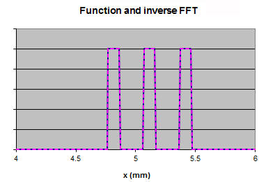
The graphs above shows f(x)^2 and FFT^2. We can now manipulate the Fourier transform and observe how this affects the inverse transform.

To change the function f(x), manipulate the mask. To calculate the Fourier transform of the new pattern, click the FFT button. To calculate the inverse Fourier transform, click the inv. FFT button. To manipulate the inverse transform, apply filters and masks in the transform column. For example, to apply low-pass filter, set everything except the central peak in the transform column equal to zero. (Click the LP Filter button.) To apply high-pass filter, set the central region in the transform column equal to zero. (Click the HP Filter button.)

[For the spreadsheet to work the "Add-Ins" Analysis ToolPak and Analysis ToolPak-VBA have to be installed and checked. The spreadsheet contains macros for the FFT and the inverse FFT. If macros are enabled, you can just click the appropriate button to calculate the FFT and the inverse FFT. If the macros do not run on your computer, click Tools, Macro, Visual Basic Editor. In the editor check that funcres.xla, procdb.xla, and atpvbaen.xla are loaded. Click Tools, Preferences, and browse for the missing files on your hard disk. You should find them in a directory with a name similar C:\Program Files\Microsoft Office\Office10\Library\Analysis.]

A low- pass filter applied to our function will yield the results shown below.