A numerical solution of the one-
dimensional, time-independent Schroedinger equation.Reference: S. E. Koonin, Computational Physics, Addison-Wesley Publishing Company Inc,
(1986).
Numerov.xlsm is a macro-enabled Excel spreadsheet
which demonstrates a method for solving the time-independent Schroedinger
equation in one dimension. This is a boundary value problem. We solve for the eigenvalues
E of the Hamiltonian for which the wave function and its derivative are
continuous and for which the wave function takes on given values at the
boundaries of the integration volume.
Numerov.m is a MATLAB function implementing the
same method.
Explanation:
We want to solve the eigenvalue equation
Hψ(x) = Eψ(x),
or
(-ħ2/(2m))∂2ψ(x)/∂x2 + U(x)ψ(x) = Eψ(x),
or
∂2ψ(x)/∂x2 - k2(x)ψ(x) = 0,
with k2(x) = (2m/ħ2)(E - U(x)).
We want to solve it in a finite region between x = -L and x = L. We assume
that in the middle of this region there exists a potential well of width a, with
a/2 << L.
Because we cannot extend our numerical solution to infinity, we
assume that U(x) = ∞ for x < -L and x > L.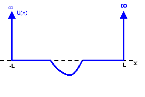
We want to find the energies for which the wave function ψ(x) and its
derivative ∂ψ(x)/∂x are continuous and the boundary conditions ψ(0) = ψ(L) = 0
are satisfied. These are the energies of the bound states of the system.
We start by expanding ψ(x) in a Taylor series expansion.
ψ(x + ∆x) = ψ(x) + ∆x*∂ψ(x)/∂x + [(∆x)2/2]*∂2ψ(x)/∂x2
+ ... .
ψ(x - ∆x) = ψ(x) - ∆x*∂ψ(x)/∂x + [(∆x)2/2]*∂2ψ(x)/∂x2
- ... .
Combining the two equations above yields
[ψ(x + ∆x) + ψ(x - ∆x) - 2ψ(x)]/(∆x)2 = ∂2ψ(x)/∂x2,
or
[ψ(x + ∆x) + ψ(x - ∂x) - 2ψ(x)]/(∆x)2 = -k2(x)ψ(x).
ψ(x + ∆x) = (2 - (∆x)2k2(x))ψ(x) - ψ(x - ∆x).
For our numerical work, let {xn} denote points on a grid defined
in the region from x = -L to x = L, n = 0, 1, …, N.
Define ψn = ψ(xn), kn = k(xn), ∆x = xn+1 - xn. Then
ψn+1 = (2 - (∆x)2kn2)ψn
- ψn-1.
We have a recipe for finding ψn+1, given ψn and ψn-1.
Integrating the wave function using this algorithm, i.e. finding its value on
the next grid point from its value at the previous two grid points, is called
integrating using the Numerov method.
We can go to the next order in the expansion
for higher numerical accuracy. Numerov.xlsm goes to 2nd order in the
expansion and numerov .m goes to 4th order.
Implementation:
To solve for the bound states of the system, we pick ψ0 = 0, ψ1
= c1, where c1 is some small number. This number c1
determines the overall normalization of the wave function. We now calculate ψ2,
ψ3, etc.
ψn+1 = (2 - (∆x)2kn2)ψn
- ψn-1.
We start integrating in the classically forbidden region,
where the magnitude of the wave function increases approximately exponentially.
As we reach the classically allowed region, the wave function becomes
oscillatory at the classical turning point. As we pass through the second
turning point and enter again into the classically forbidden region, the
integration becomes numerically unstable, because it can contain an admixture of
the exponentially growing solution. Integration into a classically
forbidden region is likely to be inaccurate. We therefore generate a second
solution, picking ψN = 0, ψN-1 = c2, and
calculating ψN-2, ψN-3, etc.
ψn-1 = (2 - (∆x)2kn2)ψn
- ψn+1.
For both integrations we pick the same value for the energy E. To determine
whether this energy E is an eigenvalue, we compare the results of our
integrations at a matching point xm in the classically allowed
region. The constant c2 is chosen so that both integrations yield
the same value ψ(xm) at the matching point and we examine the slope ∂ψ(x)/∂x
near xm. The values of E for which the slope is continuous across
the matching point are the energy eigenvalues, because for these values of E the
wave function is a solution to the Schroedinger equation which satisfies all
boundary conditions. We search for the eigenvalues by picking different values
for the energy E.
Procedure using manual matching:
Open the numerov.xlsm Excel spreadsheet It can be used to solve the one-dimensional,
time-independent Schroedinger equation for an electron trapped in various
potential wells. Sheet 1 contains the data and sheet 2 the user interface.
Examine sheet 1.
- Column A contains the position variable x in units of 10-10
m. We are going to solve the Schroedinger equation in the finite region
between x = -5 and x = 5.
- Column B contains the potential energy function U(x) in units of eV. We
are starting with a "symmetric finite square well" extending from x = -10-10
m to x = 10-10 m with a depth of 500 eV. The user interface on
sheet 2 provides us with tools to change U(x).
- Cell E2 contains a trial value for the energy E. This value can be
changes with a slider located on sheet 2.
- Colum C contains k2(x) = (2m/ħ2)(E - U(x))in units
of 1/(10-10 m)2.
With E and U(x) measured in units of eV, (2m/ħ2) has the value
2*9.11*10-31kg/(1.05*10-34 Js)2 = 1.65*10-38
J-1m-2 *(1.6*10-19 J/eV)
= 2.64 *1019 eV-1m-2 = 0.264 eV-1(10-10
m)-2.
- Column D contains the wave function ψ. It is calculated using ψn+1
= (2 - (∆x)2kn2)ψn - ψn-1
for x = -5 to x = 0.2 and using ψn-1 = (2 - (∆x)2kn2ψn)
- ψn+1 for x = 5 to x = 0.2.
- Columns I, J, and K contain different potentials that can be copied into
column B with the tools provided on sheet 2.
Switch to sheet 2.
- (i) Start with the symmetric square well with width a = 2*10-10
m and a depth of 500 eV.
Find the allowed energies for an electron trapped in this potential. How
many bound states do exist?
Note the shape of the eigenfunctions. Determine the parity of each
eigenfunction.
[In a symmetric well, i.e. a well that looks the same when reflected about a
line through its center, bound-state wave functions are either symmetric or
anti-symmetric when reflected about the same line. We say that the
symmetric wave functions have even parity and the anti-symmetric wave
functions have odd parity. In an asymmetric well bound-state wave
functions do not have a well defined parity.].
Compare the eigenvalues you found with the energy eigenvalues of the
infinite square well.
For the infinite square well we have En = n2π2ħ2/(2ma2).
If we measure a in units of 10-10 m and En in units of
eV, then En = 3.78*n2π2/a2.
- (ii) Change the well depth to 1000 eV. Find the allowed
energies for an electron trapped in this potential. How many bound
states do exist now?
- (iii) Keep the well depth at 1000 eV and change the well asymmetry to
1.5. Find the allowed energies for an electron trapped in this potential.
How many bound states do exist now? Note the shape of the eigenfunctions.
- (iv) Now choose the harmonic well. U(x) = ½kx2. Let k
= 500 eV/(10-10 m)2. For the harmonic oscillator
potential the Schroedinger equation can be solved analytically. The energy
eigenvalues are En = (n + 1/2)ħω, n = 0, 1, 2, ... . Here ω =
(k/m)1/2. (Note: The labeling of the energy levels for the
harmonic oscillator starts with n = 0, while for the square well it starts
with n = 1.)
With k measured in units of eV/(10-10 m)2 and En
in units of eV we have En = (n + 1/2)*2.76 eV*k1/2.
Numerically find the five lowest allowed energies for an electron
trapped in this potential. Determine the parity of each corresponding
eigenfunction. Compare the eigenvalues you found with the energy
eigenvalues found when solving the problem analytically.
[The harmonic well or harmonic oscillator with potential energy U(x) =
½kx2 = ½mω2x2 is one of the few
system that can be solved exactly in quantum mechanics. Most real systems
that have an equilibrium position can be approximated by a harmonic well, as
long as the average displacements from equilibrium are small and the energy
is low. It is therefore important to remember the energy levels of the
harmonic well, En = (n + 1/2)ħω = En = (n + 1/2)hf.]
- (v) Now choose the triangular well. U(x) = kx. Let k = 500 eV/(10-10
m). At x = 2, U(x) for the harmonic well above and U(x) for this triangular
well have the same numerical value.
Numerically find the five lowest allowed energies for an electron
trapped in the triangular well. Determine the parity of each corresponding
eigenfunction. Compare the eigenvalues you found with the energy
eigenvalues you found for the harmonic well. Compare the shape of the
eigenfunctions.
Procedure using programmed matching:
We numerically integrate the wave function starting at both boundaries.
For both integrations we pick E = Umin + ∆E, i.e. we pick E just
slightly larger than Umin. To determine whether the energy is an
eigenvalue, we compare the results of our integrations at a matching point xm
in the classically allowed region. We first re-normalize the wave
functions ψ1 and ψ2 obtained from our two integrations
such that ψ1m = ψ2m. We then
check if the derivatives of the two functions are equal at xm, i.e.
if dψ1(x)/dx - dψ2(x)/dx = 0.
We use dψ2 = ψ2m - ψ2m-1,
dψ1 = ψ1m - ψ1m-1.
We already have made ψ2m = ψ1m.
We therefore only have to check if ψ2m-1= ψ1m-1.
We define
f = [ψ2m-1- ψ1m-1]/ψmax.
If f ≠ 0 within a chosen limit of tolerance, then we repeat our integrations
after incrementing E by ∆E.
If f ≠ 0 for two successive iterations, but f has changed sign, then the
eigenvalue has been overshot. We decrease the magnitude and change the sign of
∆E and start decrementing E. We repeat until f = 0 within the chosen limit of
tolerance.
How do we adjust ∆E to find the value of E for which f = 0?
Pick the initial energy E1. Integrate and find f(E1).
If f(E1) ≠ 0 within a chosen limit, pick some initial ∆E to calculate
E2 = E1 + ∆E. Integrate and find f(E2). If f(E2) ≠ 0 within a chosen limit what value ∆E should pick to
find E3? Hoe do you find the root of f(E)?
If f(Ei) ≠ 0 within a chosen limit, expand f(E) about Ei.
Then set f(Ei + ∆E) = f(Ei) + df/dE|Ei∆E = 0,
where ∆E = Ei+1 - Ei.
Ei+1 is the next better value for the root of f(E).
Ei+1 = Ei - f(Ei)/(df/dE|Ei).
df/dE|Ei ≈ (f(Ei) - f(Ei-1))/(Ei - Ei-1).
Therefore
∆E = Ei+1 - Ei = -f(Ei)(Ei - Ei-1)/(f(Ei)
- f(Ei-1)).
The MATLAB function numerov.m implements programmed
matching.